Putting it altogether

Here we generate the grid, interpolate the raw bathymetry onto it and export to a SHOC readable format

NWBay TAS

%matplotlib inline
import numpy as np
from cem_gridtools.cem_gridtools import CGridRect,NN
import matplotlib.pyplot as plt
from matplotlib.ticker import FormatStrFormatter

# Load grid boundary corners from file
pts = np.loadtxt('nwbay_grid_spec.csv', delimiter=',')
x = np.array(pts[:,0], dtype='d')
y = np.array(pts[:,1], dtype='d')

#
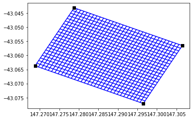
# Generate and plot gridlines
#
g = CGridRect(x,y,True)
g.gen_gridrect(100) # Cell size in metres
g.plot()

#
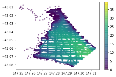
# Load raw bathy points
#
bpts = np.loadtxt('nwbay_bathy.csv', delimiter=',')
xb = np.array(bpts[:,0], dtype='d')
yb = np.array(bpts[:,1], dtype='d')
zb = np.array(bpts[:,2], dtype='d')
plt.scatter(xb,yb,s=10,c=zb, alpha=0.5)
plt.colorbar()
plt.show()

# Extract the cell centre values from the grid
xc,yc = g.get_cell_centres()
# Create the interpolant
B = NN(xb,yb,zb,"nn_sibson")
# Do the interpolation
#  Note: The cell centres need to be flattened - default ordering is 'C'
V = B.interp(xc.ravel(), yc.ravel())

#
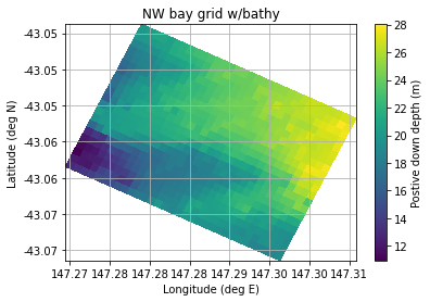
# 2D plot, note: that the interpolated depth values need to be 2D, again the default ordering is 'C'
#
Z = V.reshape(xc.shape)
plt.pcolor(xc,yc,Z)
plt.grid()
plt.title('NW bay grid w/bathy')
plt.xlabel('Longitude (deg E)')
plt.ylabel('Latitude (deg N)')
plt.colorbar(label='Postive down depth (m)')
plt.gca().xaxis.set_major_formatter(FormatStrFormatter('%.2f'))
plt.gca().yaxis.set_major_formatter(FormatStrFormatter('%.2f'))

Bathy export

Bathymetry and the shoc grid can now be exported to a text file

g.export_shoc_grid('nwbay_coords.txt')
B.export_shoc_bathy('nwbay_bathy.txt')

!head nwbay_bathy.txt

# Bathymetry
BATHY 726
19.14
18.87
18.71
18.64
18.64
19.41
19.66